The Central Limit Theorem states that the distribution of the sample means approaches normal regardless of the shape of the parent population.

Sample means (s) will normally be more distributed around (µ) than the individual readings (Xs). As n– the sample size–increases, the sample averages (Xs means) will approach a normal distribution with mean (µ).

So, don’t worry if your samples are all over the place. The more sample sets you have, the sooner the averages of those sets will approach a normal distribution with a mean of (µ).

Significance of Central Limit Theorem

The Central Limit Theorem is important for inferential statistics because it allows us to safely assume that the sampling distribution of the mean will be normal in most cases. This means that we can take advantage of statistical techniques that assume a normal distribution.

The Central Limit Theorem is one of the most profound and useful results in all statistics and probability. The large samples (more than 30) from any sort of distribution of the sample means will follow a normal distribution.

The spread of the sample means is less (narrower) than the spread of the population you’re sampling from. So, it does not matter how the original population is skewed.

• The means of the sampling distribution of the mean is equal to the population mean µ_x̅ =µ_X
• The standard deviation of the sample means equals the standard deviation of the population divided by the square root of the sample size: σ(_x̅) = σ(x) / √(n)

Assumptions

• Samples must be independent of each other
• Samples follow random sampling
• If the population is skewed or asymmetric, the sample should be large (for example, a minimum of 30 samples).

Why Central Limit Theorem is important

Central Limit Theorem allows the use of confidence intervals, hypothesis testing, DOE, regression analysis, and other analytical techniques. Many statistics have approximately normal distributions for large sample sizes, even when we are sampling from a distribution that is non-normal.

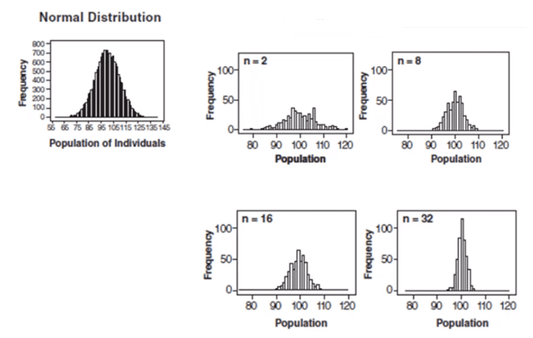
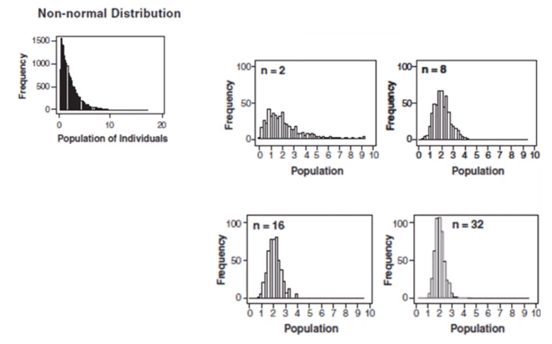
In the above graph, subgroup sizes of 2, 8, 16, and 32 were used in this analysis. We can see the impact of the subgrouping. In figure 2 (n=8), the histogram is not as wide and looks more “normally” distributed than Figure 1. Figure 3 shows the histogram for subgroup averages when n = 16, it is even more narrow and it looks more normally distributed. Figures 1 through 4 show, that as n increases, the distribution becomes narrower and more bell-shaped -just as the central limit theorem says.  This means that we can often use well-developed statistical inference procedures and probability calculations that are based on a normal distribution, even if we are sampling from a population that is not normal, provided we have a large sample size.

Unimodal Distribution

Mode is one of the measures of central tendency. Mode is the value that appears most often in a set of data values or a frequent number. The Unimodal distribution will have only one peak or only one frequent value in the data set.  In other words, Unimodal will have only one mode, the values increase first and reach to peak (i.e. the mode or the local maximum) and then decreases.

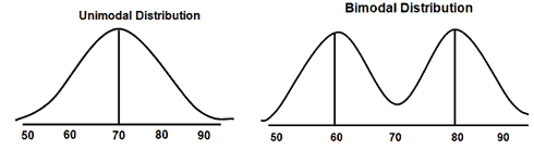
The normal distribution is the best example of a Unimodal distribution. Similarly, Bimodal distribution means there are two different modes, and multimodal means more than two different modes.

Central Limit Theorem Examples

Case 1: Less than

Example: A population of 65 years male patients with blood sugar was 100 mg/dL with a standard deviation of 15 mg/DL. If a sample of 4 patients’ data were drawn, what is the probability of their mean blood sugar being less than 120 mg/dL?

• µ = 100
• x̅ = 120
• n=4
• σ =15

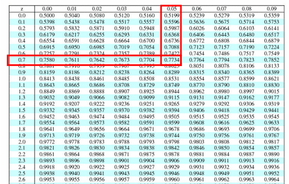
Compute P(X<120): z= x̅- µ/ σ/√n = 120-100/15/√4=20/7.5=2.66

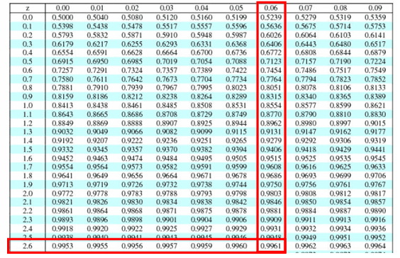
P(x<120) = z(2.66) = 0.9961 = 99.61%

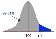
Hence, the probability of mean blood sugar is less than 120 mg/dL is 99.61%

Case 2: Between

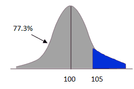
Example: A population of 65 years male patients with blood sugar was 100 mg/dL with a standard deviation of 20 mg/DL. If a sample of 9 patients’ data were drawn, what is the probability of their mean blood sugar being between 85 and 105 mg/dL?

First, compute P(x<105)

• µ = 100
• x̅ = 105
• n=9
• σ =20

Compute the Z score z= x̅- µ/ σ/√n = 105-100/20/√9=5/6.67=0.75

P(x<105) = z(0.75) = 0.7734 = 77.3%

Then, compute P(x<85)

• µ = 100
• x̅ = 85
• n=9
• σ =20

Compute the Z score z= x̅- µ/ σ/√n = 85-100/20/√9=-15/6.67=-2.24

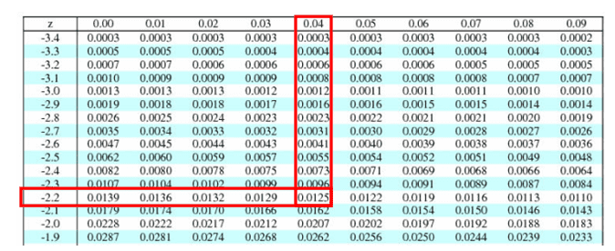
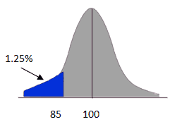
P(x<85) = z(-2.24) = 0.0125 = 1.25%

Since we are looking for blood sugar between 85 and 105 mg/dL P(85<x<105) = 77.3-1.25 = 76.05%

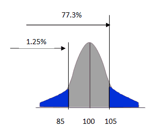
Hence, the probability of mean blood sugar is between 85 and 105 mg/dL is 76.05%

Case 3: Greater than

Example: A population of 65 years male patients with blood sugar was 100 mg/dL with a standard deviation of 20 mg/DL. If a sample of 16 patients’ data were drawn, what is the probability that their mean blood sugar is more than 90 mg/dL?

• µ = 100
• x̅ = 90
• n=16
• σ =20

Compute the Z score z= x̅- µ/ σ/√n = 90-100/20/√16=-10/5=-2

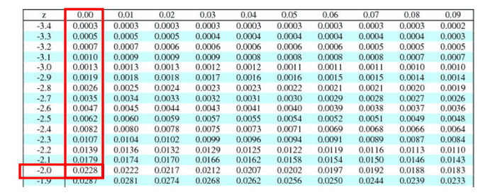
P(x<90) = z(-2.0) = 0.0228 = 2.28%

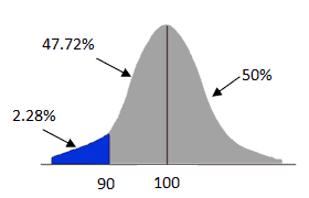
Since we are looking for blood sugar of more than 90 mg/dL =100%-2.28%=97.72%

Hence, the probability of mean blood sugar greater than 90 mg/dL is 97.72%

Jarque- Bera analysis.

Wikipedia has a good article here:

Central Limit Theorem Videos