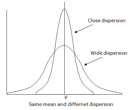
Dispersion is the degree of variation in the data. In other words, the extent of the spread of values from the mean. Items in a data set tend to differ from each other and the mean. So, dispersion measures the extent to which different items tend to disperse away from the central tendency.
The measure of central tendency gives the central value around which all the values spread along with the central value, but that does not give the correct picture of the variability of the data.
The better method to find the spread or scatter of the data is the measure of dispersion. It attempts to quantify the variability or spread of the data. The measure of dispersion tells how the data spreads or scatters around the center value. Dispersion is nothing but “distance from the average”.
Why Measure of Dispersion Is Important
For Example, Set-1 household income data is $70K, $60K, and $50K respectively; the average is $60K. Set-2 household income is $20K, $50K, and $100K; the average is $60K.
Dispersion indicates the extent of uniformity. Uniformity and degree of variation are inversely proportional. In other words, more uniformity, less variation. From the above example, though the average salary of the two sets is the same ($60K), the first set of household data indicates more uniformity. Similarly, the second set of data shows more variation around the center.
If the means of two or more series are the same, do not think of them as similar because their other characteristics (dispersion, skewness, kurtosis), may differ. Hence, the method of dispersion helps to find the correct variation of the data.
Objective of Dispersion
- To determine the reliability of an average
- Compare two or more data sets with regard to the variability
- Facilitate computations of other statistical measures
- To indicate the level of uniformity of variables
Different types of Measures of Dispersion
There are several measures of dispersion, the most common being are
- Range
- Variance
- Standard Deviation
- Coefficient of Variation
- Inter Quartile range
Range
Range is the difference between the maximum and the minimum value.
Example: The age of the randomly sampled audience in a theatre is 55, 16, 23, 65, 45, 34, 28, 37, 58, and 24. Find the Range.
Arrange the values in ascending order: 16, 23, 24, 28, 34, 37, 45, 55, 58, 65
Range = Maximum-Minimum = 65 -16 = 49
- The range can be used with ordinal or interval ratio variables but cannot be used with a nominal scale.
- The disadvantage of Range – it completely depends upon the extreme values. Thus, the range is affected by the outliers.
Variance
Variance measures the dispersion of a set of data points around their mean value.
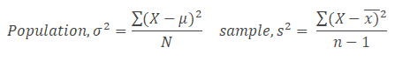
Population variance, denoted by sigma squared, is equal to the sum of squared differences between the observed values and the population mean, divided by the total number of observations.
Sample variance is denoted by s squared and is equal to the sum of squared differences between observed sample values and the sample mean, divided by the number of sample observations minus 1.
Standard Deviation
Standard Deviation is the most popular measure of dispersion. The symbol for the measurement of dispersion in a population is denoted by the Greek letter sigma σ. Similarly, the sample standard deviation denoted by s (or sd) is a point estimate for the population standard deviation / the dispersion statistic for samples.
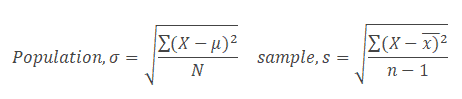
Standard deviation is the positive square root of the arithmetic mean of the squares of the deviations of all the observations from their mean.
Unlike range, the standard deviation takes each data point into account while calculating the dispersion.
The lower the standard deviation, the lower the process variability. In other words, data points are closer to the mean or average value.
Example: Determine the standard deviation of the weights (in lbs) of 12 samples.

n =12 and n -1 =11
Average of 12 samples X̅= ΣX/n = 1848 / 12 = 154
Compute the deviation i.e (X-X̅) and then square each deviation (X-X̅)2
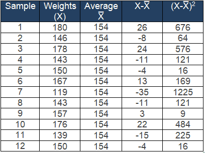
Sample standard deviation s= √Σ(X-X̅)2 / n-1 = √3702 / 11 = 18.3
s is the standard deviation of the sample (18.3) which is used as an estimate for the population from which the sample was taken.
Coefficient of Variation
The Coefficient of Variation is the standard deviation relative to the mean. In other words, the Coefficient of Variation is equal to the standard deviation divided by the mean, and it is expressed as a percentage. It is also known as relative standard deviation.
COV = s/ X̅ * (100%) or COV = σ / µ * 100%
Example: From the above example s = 18.3 and X̅ = 154
Coefficient of Variation COV = s/ X̅ * (100%) = 18.3 / 154 * 100 = 11.9%
Inter Quartile range
Inter quartile range is one of the measures of dispersion. It is defined as the difference between the first and third quartiles.
IR = Q3 – Q1
Example: Find the Inter Quartile range of 10 students’ marks in a science subject.
56, 78, 35, 89, 92, 52, 66, 72, 84, 96
- Arrange the values in ascending order
- 35, 52, 56, 66, 72, 78, 84, 89, 92, 96
- n=10
- Calculate Q1 = ¼ (n+1) = 11 / 4 = 2.75th term = 52 + (0.75) * (56 – 52) = 55
- Calculate Q3 = ¾ (n+1) = 3 * 11 / 4 = 8.25th term = 89 + (0.25) * (92 – 89) = 89.75
Inter Quartile range = Q3-Q1 = 89.75 – 55 = 34.75
Kurtosis
Kurtosis is a statistical measure to determine whether the data are heavy-tailed or light-tailed relative to a normal distribution. In other words, Kurtosis is a measure of the thickness of the tails of a distribution.
Kurtosis is a measure of the peakedness of a distribution. The larger the kurtosis, the more peaked the distribution. The standard normal distribution has a kurtosis of 3.
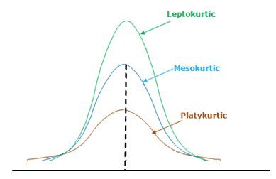
There are three types of Kurtosis
- Leptokurtic: It is a curve having a high peak than the normal curve. Too much concentration of the items near the center. Leptokurtic distribution has positive kurtosis values. Most financial returns are Leptokurtic.
- Platykurtic: It is a curve having a low peak (flat) than the normal curve. There is less concentration of items near the center. A platykurtic distribution shows a negative excess kurtosis.
- Mesokurtic: It is a curve having a normal peak or the normal curve. There is an equal distribution of items around the center values. Mesokurtic has zero value kurtosis value. In other words, Mesokurtic is the same as the normal distribution.
What is Excess Kurtosis?
It is a metric that compares the kurtosis of a normal distribution to the kurtosis of a distribution. The normal distribution kurtosis value is 3.
Hence, Excess Kurtosis = Kurtosis – 3.
Related notes on Dispersion:
We need six points (strata, units of measure) under the upper control limit of the range in order to have sufficient measurement discrimination. This is due to rounding. Too much rounding causes a loss of information about dispersion in a sample.
http://www.six-sigma-material.com/Measures-of-Dispersion.html (Measures of Dispersion)