Normal Distribution (AKA Gaussian Probability Distribution)

The Normal distribution is used to analyze data when there is an equally likely chance of being above or below the mean for continuous data whose histogram fits a bell curve. Statisticians refer to the normal curve as the Gaussian Probability Distribution, named after Gauss.

Entertainingly, when students ask for a professor to grade on a curve, they probably don’t know that would mean 50% of the students would receive below a 50 or less than a D!

Basic Assumptions:

Normal Distribution is the most widely known symmetric distribution for continuous data.
Symmetrical distribution about the mean (a bell-shaped curve)
- They will never be perfect unless you have an infinite data set.
Commonly used in inferential statistics.
- This is often the most used distribution in Six Sigma.
Family of distributions described by m and s
The peak of the normal curve indicates the average, which is the center of process variation. An average of a group of numbers indicates the central tendency.
If there is a normal curve, then there is no undue influence in the process.
Is symmetric:
- Many other distributions can be symmetric under the right conditions, including Binomial & Chi Square.
- Do NOT assume that symmetric data is normally distributed.

When to Use Normal Distribution

When data is grouped around the mean, there is an equal probability of being above or below the mean (50% above & 50% below the average).
If we can transform data to behave like a normal distribution, then we do it! Much easier to work with data in this shape.
- Ex. If we have to take the log of values or subtract a number or perform some other operation on the data, then do it.
Use when the histogram fits a bell curve.
Use when the goodness-of-fit statistic is less than the selected P-value (usually 0.05).

Uses Include:

A Normal Distribution is used to test population means from sample data.
Use a histogram to determine if data are normally distributed.
Probabilistic assessments of the distribution of time between independent events taking place at a constant rate.
The shape can be used to describe constant failure rates as a function of usage.
The standard normal or t-distributions are most likely used to compare two process means.

Formulas for Standard Normal Distribution

In a normal distribution, 68% of the data will occur within +/- 1 standard deviation.

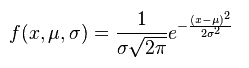
e = constant (2.71828) – Poisson constant
x = control variable – (data being studied)
µ = population mean
σ = population standard deviation

Formulas for Population mean, Variance, and Standard Deviation.

Formula for Population Mean, Variance, Standard Deviation

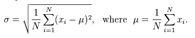
N (capital N) refers to Population.

In this case, σ^2 is the variance.

Formulas for Sample mean, Variance, and Standard Deviation.

Formula for Sample Mean, Variance, Standard Deviation — Formula for Sample Mean, Variance, and Standard Deviation

n (lowercase n) refers to sample size.

In this case, s^2 is the variance.

The population equations differ from the sample equations because we wish to reduce the “degrees of freedom” or increase our confidence in the sample.

Variation and Bell Shape

Adjusting to Center

You do not want to adjust an ongoing process to “center it.” This increases variation. The more you do this, the more the operator unduly influences the process, and the less the distribution will be shaped like a bell. See Quincunx demonstration.

Center of Process Variation

The peak of the normal curve indicates the average, which is the center of process variation.

5Ms & 1 P

When you have a bell-shaped curve, none of the 5 Ms or one P are unduly influencing the process.

Additional Notes:

Normal Distribution Videos

Good basic description of normal distribution

What is a standard normal distribution?

ASQ Six Sigma Black Belt Certification Normal Distribution Questions:

Question: For a normal distribution, two standard deviations on each side of the mean would include what percentage of the total population? (Taken from ASQ sample Black Belt exam.)

Answer:

Unlock Additional Members-only Content!

To unlock additional content, please upgrade now to a full membership.
Upgrade to a Full Membership
If you are a member, you can log in here.

Thank You for being a Member!

Here’s some of the bonus content that is only available to you as a paying member.

A: 95%. For this question, you need to remember that nearly all of a process’s outputs will be within 6 sigmas – or 6 standard deviations. 2 standard deviations on each side of the mean would be 95% of all outcomes.

Comments (4)

In paragraph two you describe “grading on a curve,” but traditionally schools (especially law schools) centered the curves at mid-C with 10% getting an A and 10% getting an F. This technique is seldom used outside of law schools and when it is it is generally centered at a slightly higher point (such as a low B) due to grade inflation that we’ve seen over the last 40 years. If you wanted to, including information on this might be fun. What you have already gets the important point across to the reader. Before I move on though, here are two examples of “grading on a curve.”

40 years ago my mother received an “A-” with a raw grade of a 96% since the class average of the raw grades was a 92%. In contrast however that same year my father received a “C+” in an engineering course for earning a raw grade of 26% since the class average was a 24%.

The very bottom of the page made me think about the different ways of measuring the center of the data. A reader who has gotten that far should already know about the mean, median, and mode, but if you have a page on that it wouldn’t hurt to include a link just in case a reader is interested.

Six Sigma seems to be heavily focused on the use of the Normal Distribution but broader certifications such as the ASQ Quality Engineering certification dive quite deeply into non-normal distributions as well as ways of measuring deviation from normal (skewness and heavy shoulders versus heavy tails). Although I personally don’t consider skewness and heavy shoulders vs heavy tails to be an “advanced topic,” it appears that Six Sigma treats it as such, and thus it probably isn’t really needed on this page. It might be an idea for something to add someday later though.

Great notes, Jeremy.

I do have a basic statistics page that I am building here. It will include mean, median, mode, and a few other items that are necessary to understand graphical analysis and data analysis in Six Sigma.

As for non-normal distributions, that is a fair point. Things work better when we can assume a normal distribution. And aside from a few select instances, if your process is not reflecting a normal distribution, and it cannot be transformed to a normal distribution, then you have to wonder if the process is really in control or if there are factors like common cause or special cause variation that are making it so. If you really do have to work with non-normal data, you would apply one of the following non-parametric tests.